Decision Tree and Interpretation on Telecom Data

We saw that logistic Regression was a bad model for our telecom churn analysis, that leaves us with Decision tree.

Again we have two data sets the original data and the over sampled data. We run decision tree model on both of them and compare our results.

So running decision tree on the normal data set yielded better results as compared to running on the over sampled data set

	Accuracy	Kappa	Precision	Recall	Auc
Data	0.9482	0.7513	0.68421	0.90698	0.837
Over Sampled Data	0.8894	0.5274	0.5965	0.5862	0.7656

Unfortunately the decision tree plot was too big for me to put it in this post.

As decision tree is giving the highest level of accuracy , we will select it as the clear winner for our telecom churn analysis problem.

Another major advantage of decision tree is that it could be explained graphically very easily to the end business user on why a particular choice is being made.

You can find the code for decision tree here->

https://github.com/mmd52/Telecom_Churn_Analysis/blob/master/Decision_Tree.R

This was a dummy database and may not have yielded the best results , but is a perfect exercise for practice.

Logistic Regression And Interpretation On Telecom Data

If you have read my previous posts, you may have understood how feature engineering was done and why we are running a logistic regression n this data.

It is essential to understand we have two train sets

1. The original train set
2. The over sampled train set

Running Logistic regression on the normal data set yielded the following results

#Accuracy 87.53%
#Kappa 0.275
#Precision 22.807%
#Recall 0.59091 %
#AUC 0.602

Now running logistic regression on the over sampled data yielded the following results

#Accuracy 84.71 %
#Kappa 0.3265
#Precision 0.40351
#Recall 0.42593
#AUC 0.660

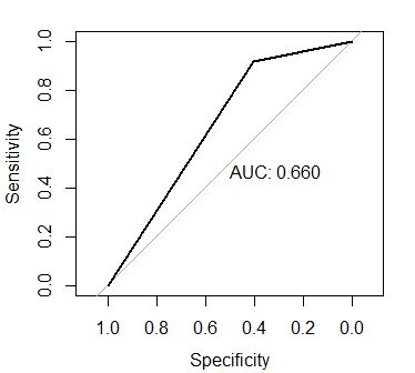
From both the models we can see when we use auc as our metric the over sampled data is clearly the winner. Also we will rely on the second model more because the kappa value is higher and precision recall values are closer.

One massive problem thanks to null deviance we face is that our accuracy after running our best model is 84.71% ; And our accuracy by running no model and stating customer retained is 85.8%. Means our model is not as effective as we would think. This means we either should try feature engineering or a different model.

As this data is falsified could be that our accuracy will always be bad, but lets assume logistic yielded a good result, let us try to understand the equation then,

Coefficients:
 Estimate Std. Error z value Pr(>|z|) 
(Intercept) 8.318e+00 1.078e+00 7.713 1.23e-14 ***
StateAL 1.767e-02 5.858e-01 0.030 0.975929 
StateAR -6.454e-01 6.095e-01 -1.059 0.289611 
StateAZ 6.812e-01 6.998e-01 0.973 0.330355 
StateCA -2.015e+00 5.959e-01 -3.382 0.000719 ***
StateCO -5.204e-01 5.958e-01 -0.873 0.382438 
StateCT -9.923e-01 5.768e-01 -1.720 0.085364 . 
StateDC -7.558e-01 6.655e-01 -1.136 0.256046 
StateDE -8.036e-01 5.780e-01 -1.390 0.164413 
StateFL -5.576e-01 5.832e-01 -0.956 0.339026 
StateGA -8.233e-01 5.512e-01 -1.494 0.135263 
StateHI 3.252e-01 7.279e-01 0.447 0.655050 
StateIA 2.778e-02 7.161e-01 0.039 0.969051 
StateID -4.276e-01 5.647e-01 -0.757 0.448895 
StateIL -1.270e+00 5.720e-01 -2.220 0.026441 * 
StateIN -7.517e-01 5.884e-01 -1.278 0.201372 
StateKS -1.164e+00 5.425e-01 -2.145 0.031918 * 
StateKY -7.379e-01 6.068e-01 -1.216 0.223949 
StateLA -1.080e+00 5.963e-01 -1.811 0.070173 . 
StateMA -1.541e+00 5.610e-01 -2.746 0.006032 ** 
StateMD -1.164e+00 5.565e-01 -2.092 0.036455 * 
StateME -1.915e+00 5.471e-01 -3.500 0.000465 ***
StateMI -1.501e+00 5.746e-01 -2.612 0.009011 ** 
StateMN -8.528e-01 5.486e-01 -1.555 0.120064 
StateMO 2.519e-01 6.291e-01 0.400 0.688826 
StateMS -1.467e+00 5.614e-01 -2.613 0.008987 ** 
StateMT -1.447e+00 5.473e-01 -2.644 0.008181 ** 
StateNC -8.929e-01 5.817e-01 -1.535 0.124820 
StateND -6.750e-01 6.037e-01 -1.118 0.263526 
StateNE -6.011e-01 5.911e-01 -1.017 0.309221 
StateNH -8.939e-01 6.064e-01 -1.474 0.140435 
StateNJ -1.738e+00 5.556e-01 -3.128 0.001761 ** 
StateNM -1.151e+00 5.471e-01 -2.104 0.035366 * 
StateNV -1.757e+00 5.525e-01 -3.180 0.001473 ** 
StateNY -1.080e+00 5.650e-01 -1.912 0.055908 . 
StateOH -5.434e-01 5.577e-01 -0.974 0.329891 
StateOK -1.484e+00 5.837e-01 -2.543 0.011001 * 
StateOR -4.159e-01 5.561e-01 -0.748 0.454572 
StatePA -8.248e-01 6.262e-01 -1.317 0.187836 
StateRI 4.828e-01 6.553e-01 0.737 0.461271 
StateSC -1.327e+00 5.734e-01 -2.313 0.020695 * 
StateSD -1.419e+00 5.936e-01 -2.390 0.016838 * 
StateTN -2.747e-01 5.931e-01 -0.463 0.643201 
StateTX -2.148e+00 5.466e-01 -3.929 8.53e-05 ***
StateUT -7.398e-01 5.785e-01 -1.279 0.200914 
StateVA 7.518e-01 6.311e-01 1.191 0.233547 
StateVT -4.988e-01 5.869e-01 -0.850 0.395327 
StateWA -1.369e+00 5.698e-01 -2.402 0.016308 * 
StateWI -2.333e-01 5.906e-01 -0.395 0.692830 
StateWV -4.497e-01 5.560e-01 -0.809 0.418600 
StateWY -1.921e-01 5.780e-01 -0.332 0.739637 
Account_Length -1.719e-03 1.189e-03 -1.446 0.148198 
Area_Code 1.860e-03 1.085e-03 1.714 0.086489 . 
Phone_No -1.627e-07 1.687e-07 -0.964 0.334881 
International_Plan yes -2.516e+00 1.206e-01 -20.858 < 2e-16 ***
Voice_Mail_Plan yes -1.028e-01 1.447e-01 -0.710 0.477407 
No_Vmail_Messages -2.941e-03 5.303e-03 -0.555 0.579144 
Total_Day_minutes -4.437e+00 2.775e+00 -1.599 0.109815 
Total_Day_Calls 3.982e-05 2.389e-03 0.017 0.986701 
Total_Day_charge 2.603e+01 1.632e+01 1.595 0.110808 
Total_Eve_Minutes -1.862e+00 1.418e+00 -1.313 0.189311 
Total_Eve_Calls -4.211e-03 2.379e-03 -1.770 0.076674 . 
Total_Eve_Charge 2.182e+01 1.668e+01 1.308 0.190938 
Total_Night_Minutes 9.630e-01 7.453e-01 1.292 0.196293 
Total_Night_Calls -6.086e-04 2.392e-03 -0.254 0.799175 
Total_Night_Charge -2.143e+01 1.656e+01 -1.294 0.195715 
Total_Intl_Minutes 2.219e+00 4.482e+00 0.495 0.620579 
Total_Intl_Calls 1.075e-01 2.053e-02 5.233 1.67e-07 ***
Total_Intl_Charge -8.763e+00 1.660e+01 -0.528 0.597585 
No_CS_Calls -5.475e-01 3.540e-02 -15.466 < 2e-16 ***
---

Cant read it ? well think you just made this model and your boss calls up and asks you, there is a customer his state his NV his total calls, charges and duration is xyz , Will he leave the telecom operator? if yes please explain?

What will you say , well its easy you look at the above table and start. Every factor that your boss gave fits in the equation and you could quantitatively justify your answer. All of this thanks to the historical data.

For simplicity lets consider equation

y = 45    +  60*(age)
where y=salary
45=intercept

How would you interpret this equation, it obvious you would say as age increases , so does salary increase. right?

How ever think again and think hard this time, what if I told you age is 0? Now explain it to me? Im sure you understood here that a newborn cannot have a salary of 45 $ without doing anything. This is where business understanding or domain knowledge comes into play.

We should usually avoid explaining the intercept unless the business understanding , helps you to explain it. But this is a Gray area, so its better to avoid explaining it , then to make a mess out of it.

However imagine if this same equation was for a packet of wafers

y = 45 + 0.1(weight)

Here we could simply say that mean weight that should be in a packet of wafers is 45 gms, however that is not always true so a variance factor in the form of coefficients is added.

That is why intercept at some places could be explained and some places cannot be.

You can find the code for logistic regression Here ->

https://github.com/mmd52/Telecom_Churn_Analysis/blob/master/Logistic_Regression.R

Determining Feature Importance For Telecom Data

We have a complete data set  -> Check

Feature engineering done -> Check

How many variables do we have?    20 variables

How many should we ideally use ?   Not more that 10 ideally

How to determine which variables to include and which not to ?   Its simple do Boruta!!

Whats Boruta?

Boruta is a feature selection algorithm. Precisely, it works as a wrapper algorithm around Random Forest. You can read about it here ->  https://www.analyticsvidhya.com/blog/2016/03/select-important-variables-boruta-package/   Analytics vidhya has given a pretty good explanation about it here.

Now keep one important thing in mind we have two train sets 1)Normal train set  2)Smote Train set.

So upon running boruta on the normal train set, boruta confirmed the variables International_Plan,Voice_Mail_Plan ,No_Vmail_Messages,Total_Day_minutes,
Total_Day_charge,Total_Eve_Minutes,Total_Eve_Charge,Total_Night_Minutes,
Total_Night_Charge , Total_Intl_Minutes,Total_Intl_Calls,Total_Intl_Charge,
No_CS_Calls as important.

And upon running Boruta on Smote data set, Boruta confirmed all the variables as important, you can find the boruta code below

https://github.com/mmd52/Telecom_Churn_Analysis/blob/master/Boruta_Imp_FE.R

Feature Engineering On Telecom Data

Although the Telecom data provided by https://www.sgi.com/tech/mlc/db/ has no missing values , there is a landslide of class imbalance.

That is why the only thing we will concentrate in our feature engineering is eliminating class imbalance.

> summary(train$Customer_Left)
False True 
 2850 483

Its Visible that retained customers in our training set is 2850 and customer who left are 483. Because of this I will do oversampling on the customers who left to balance the data set.

Let us assume that I do not over sample , then by even not making any model I can simply say customer retained and still be right 85.8% of the time. In order to break this bias I use a package known as SMOTE(Synthetic minority oversampling technique ) you can read about the research paper published in the Journal of Artificial Intelligence Research 16 (2002) here -> https://www.jair.org/media/953/live-953-2037-jair.pdf

> train$Customer_Left<-as.numeric(train$Customer_Left)
> summary(as.factor(train$Customer_Left))
 1 2 
 483 2850 
> train$Customer_Left[train$Customer_Left==2]<-0
> summary(as.factor(train$Customer_Left))
 0 1 
2850 483  
#here false ->1
# true ->0
> train$Customer_Left<-as.factor(train$Customer_Left)
> ntrain<-SMOTE(Customer_Left~.,train,perc.over=200,k = 3)
> ntrain$Customer_Left<-as.factor(ntrain$Customer_Left)
> summary(ntrain$Customer_Left)
 0 1 
1932 1449

Now we have simply under sampled retained customers from 2850 to 1932 and over sampled customers who left the operator from 483 to 1449.

Now train has been manipulated hence I also had to manipulate test once.

You can see the complete code here ->  https://github.com/mmd52/Telecom_Churn_Analysis/blob/master/FE.R

NOTE-> The libararies.R file consists code that loads packages needed and if they are not installed on your machine it will download and then install them.

Churn Analysis On Telecom Data

One of the major problems that telecom operators face is customer retention. Because of which majority of the Telecom operators want to know which customer is most likely to leave them, so that they could immediately take certain actions like providing a discount or providing a customised plan, so that they could retain the customer.

However accuracy required while building a churn analysis model needs to be very high, imagine if our model has a accuracy of just 75% and the total number of customers who want to leave are just 5% , this leaves a margin of 20% of customers who were wrongly classified as customers who will leave the operator. If an operator has 10000 customers,And 2500 customers are predicted to leave , the operator may have to release lets assume a 1$ credit to all that’s a cost of 2500$, where as credits that required to be released was only for 5% of the customer’s that is a cost of 500$, hence the operator spent 2000$ for no reason. If the operator has high number of customers it would lead to a huge loss.

Coming to the data quotient, there is no freely available telecom data as far as I know available, however the website https://www.sgi.com/tech/mlc/db/ provides data for churn analysis, this data is not real but represents real world scenarios and is good from the perspective of understanding and learning.

The data on the website is classified into train and test has no NA’s means no feature engineering as such to be done before running models on it.

Now comes the question of which models to run on it. Some would say since we need very high accuracy hence we will run xgboost or random forest, however the downside we have here is that we cannot explain to the operator on what basis is XGBOOST or random forest determining why will the customer leave him. Even if we manage to explain its very complicated and will not be accepted.

Because of this we will have to take support on models that can be easily explained to the customer. This leaves us with two models for classification .i.e. customer leaves -> 0 or customer is retained -> 1. So the models are Logistic regression and decision tree.

Why Logistic Regression ?  well because we can explain to the operator why customer is leaving him thanks to the logit equation.

Why Decision Tree? well because there is a neat flow of how our tree makes decision by breaking variables and deciding yes and no based on entropy and impurity.

Further in this post category I will show feature engineering to Running models, to interpretation.

The data available from the website is a bit complex to save to a CSV file so if you need you can download the train and test data from below.

Also explanation of variables is not provided as it is fairly simple.

https://github.com/mmd52/Telecom_Churn_Analysis